What we know we don’t know about algorithms
I believe we, developers, have started to forget the importance of algorithms that reside at the core of what we do. They are hidden beneath frameworks and libraries, mischievously eluding our awareness as we are caught up with daily tasks. I will try to persuade you that paying attention to them, taking a step back to classify the problem at hand from the algorithms perspective can make the difference between failure and success, between software masterpiece and technical debt. That being said, let us dive into it. First, what is an algorithm?
According to Google, it is “a process or set of rules to be followed in calculations or other problem-solving operations, especially by a computer.” According to Wikipedia, it is “a finite sequence of rigorous instructions, typically used to solve a class of specific problems or to perform a computation“. In that regard, it is common knowledge that adding two numbers is not an algorithm. Neither is Ubuntu operating system. There must be something in between which is not trivial, and which also has a bound scope. Something you can apply to multiple situations, and you can use to classify and understand problems. What algorithms do you think of when someone asks you to name one?
Let us start with the first ones and build up from there. It is difficult to settle the starting point of algorithms, but few dare to go back to before the ancient Babylonian clay tablets. Recently decoded, they contain Pythagorean numbers written in base 60 (from where we have our base for time measurements and angles measured in degrees (Babylonians years had 360 days, as the Earth covers approximately 1 degree each day around the Sun, conveniently for their 60 number bases).

However, numbers and techniques to draw a right angle can hardly be named “algorithms”, that is why some say it is Eratosthenes with his Sieve, discovering a method for finding all prime numbers (up to a certain limit) while measuring the circumference of the Earth and being the chief librarian at the Library of Alexandria.

I personally prefer to place the birth of algorithms in the hand of Euclid, probably the most influential figure in the history of mathematics, as the father of geometry (through his work in “Elements”, still the second most published book after the Bible). Also in the Elements, an idea that is now called the fundamental theorem of arithmetic started what is now the number theory, stating that every (integer) number has a unique prime factorization, which makes prime numbers the building blocks of all numbers.

Even for ancient Greeks, primes were more than an interesting curiosity. Using the theorem above, they were providing an effective way to simplify fractions, which was especially useful in constructions (or splitting goods). Because it was cumbersome to decompose the nominator and denominator into its prime factors and perform simplifications this way, Euclid devised an algorithm to compute the greatest common divisor of two numbers (gcd function) efficiently. If you did any computer science, it is that one of the first algorithms you implemented was the gcd or the primality test.
If we allow ourselves a quick time travel jump 2500 years in the future, this is how gcd algorithm might look like in java.

Muhamad ibn al-Khwārizmī
It can be argued that the history of algorithms starts with Muhamad ibn al-Khwārizmī, a Persian mathematician that lived in Bagdad in the 9th century. The word “algorithm” is derived from his name. He was the one who introduced decimal positional system to the world, in his book “On calculation with Hindu numerals”. It is not for this book that we call him the father of algorithms however, but for a book that was requested of him by the Caliph, in which he had to compile a list of daily life problems and methods for solving them. This included, among other things, questions about the measurement of land, commercial transactions, and distribution of a legacy in the family. He decided to start the book with a mathematical work that would abstract all concrete problems into what we now call algorithms. The famous book is called “The Compendious Book on Calculation by Completion and Balancing”. In Arabic, that would be “al-Kitāb al-Mukhtaṣar fī Ḥisāb al-Jabr wal-Muqābalah” but the shorter version is known as al-Jabr, which we now simply call algebra, after the book that established the new mathematical field.

Ada Lovelace and the Generation of Bernoulli series algorithm
Some argue that to have an algorithm, one needs a machine to run it. If humans do it by hand, it is mere mathematics. Those will set the birthplace of algorithms in 1843, in a publication written by Ada Lovelace to prove the usefulness of a mechanical machine designed by Charles Babbage which he called Analytical Engine. In Ada Lovelace notes to Sketch of The Analytical Engine Invented by Charles Babbage by Luigi Menabrea she described how the Analytical Engine could calculate the Bernoulli numbers using a recursive algorithm, that could run on a machine that has never been built. Bernoulli numbers appear when calculating any sum of powers of natural numbers. Having a formula for them simplifies calculus. They are also connected to prime numbers and provide a way to distinguish between regular and irregular primes. As we will also see later, primes are following us everywhere. You can read more about Ada Lovelace algorithm and history here.
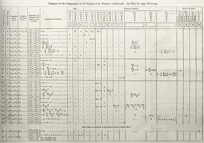
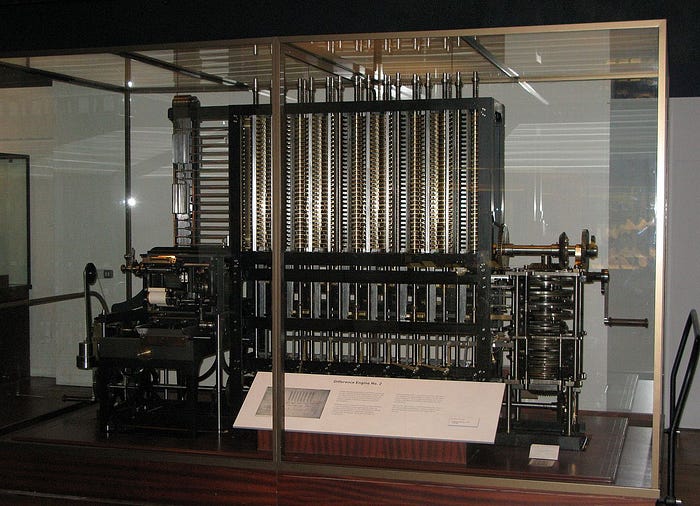
The analytical engine was never built, as it was not feasible at that time to produce mechanical components at such a high precision and quality as needed, but two difference engines (v2) were built, one by the Science Museum in London in the 80' and another one in US which is now at Intellectual Ventures in Seattle. Luigi Menabrea paper along with Ada Lovelace first complex algorithm designed for a machine uncovered the possibilities of computing machines, fueling what has become the era of computing. Below, you can see the marvelous first difference engine built, a machine of 8,000 parts and weighing about 5 tons. As Menabrea cleverly intuited, in the future, mathematicians will no longer be needed for complex calculus. Workmen should do simply fine. We, the programmers, are the “workpeople” working on these machines, and indeed, we are no mathematicians.
When once the engine shall have been constructed, the difficulty will be reduced to the making of the cards; but as these are merely the translation of algebraic formulae, it will, by means of some simple notation, be easy to consign the execution of them to a workman. — Italian engineer and future prime minister Luigi Menabrea on the design of Analytical engine
Soon after, Alan Turing came along and proposed a Universal Turing Machine that can compute everything, inspiring the construction of electronic programmable computers. In Alan Turing theoretical design, the Turing Machine was the program (the algorithm), past to the Universal Turing Machine along with the input. This gave a new dimension to programmability and defined terms like algorithm and computability in mathematical terms, as he was disproving the decidability statement of David Hilbert’s program, of formalizing mathematics. Along with Kurt Gödel’s completeness theorem, we now know that, unfortunately, mathematics is neither complete nor decidable, but the byproduct of Turing’s proof, the Turing Machine, gave birth to computer science as we know it and to the information age that followed. He really is our role model and our founding parent for this achievement.
Immediately after, algorithms penetrated every field of our existence, detecting, searching, classifying, modeling, predicting, reporting, and optimizing everything from the next best chess move to next best time interval for the green traffic light, into human behavior understanding and persuasion, theorem proving and protein unfolding. Let us see how we can classify them to shed some light on the possibilities and methods offered by algorithms.
Classification: Recursive vs iterative algorithms
Remember the Euclid algorithm at the beginning of the article? There is another way to solve this problem, which I’m sure you will recognize instantly:
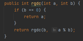
It is the recursive version of the same algorithm that you can see above which brings us to one of the ways we can devise algorithms: Iterative and recursive. In theory they are equally valid, in practice we might prefer the iterative approach as each method call consumes some memory on the stack on each call (in Java at least). The algorithm above is a special case of recursion: it is tail-recursive, and in most functional programming languages today it is optimized by the compiler. That can be a good reason to use Scala or Kotlin instead of Java if you plan to use recursion in your code. On the deeper level, the existence of the stack and of the compiler behind every programming language function makes each recursive function, in principle, an iterative one. Remember that in principle it runs on something like a Turing machine.
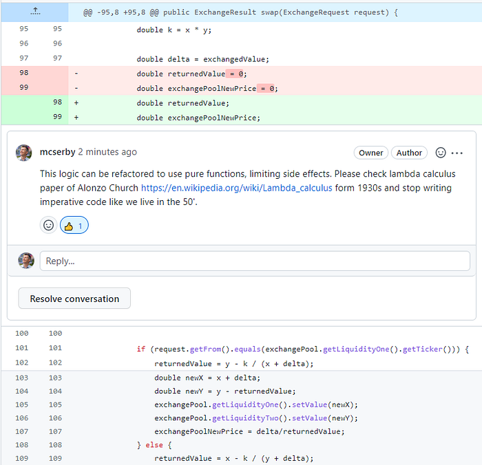
Every recursive algorithm can be expressed iteratively and vice versa, and that is a fact. We know that because in the ’30s, three computational models have been defined: Kurt Godel’s general recursive functions, lambda calculus (introduced by Alonzo Church) and Turing machines, introduced by, of course, Alan Turing, which have been proven to be equivalent. These three gentlemen made life difficult for you, the developer, as if you are asked to convert a recursive function into its equivalent iterative variant (as some projects or companies forbid recursivity) you cannot tell them it is not possible. Moreover, if you are an imperative style programmer and the team lead adds a comment in your pull request stating that “this can be implemented with pure functions to limit side effects” it has already been proven that it can be done (yes, even in Java), you just need to figure out how.
We now say that something is computable by definition if it can be implemented by a Turing machine. We do not know yet if any function is computable (by a Turing machine), as we do not yet know what an “effectively calculable” function is or can be outside of Turing’s definition. From a practical point of view, we believe that every function which does not involve infinite loops is computable, so you cannot use this argument to tell your stakeholder that his requested feature is impossible to implement. There are, of course, problems that are undecidable, problems for which there cannot be any algorithm we can write to solve. The most famous example is Alan Turing’s Halting Problem, stating that there cannot be an algorithm that can determine if a given algorithm (or Turing Machine) and an input produces a result or runs indefinitely. For this sort of problem, let us suppose that your stakeholder asks you to implement a code generation algorithm that optimizes the company budget. In that case, you should start with a huge “spike” to research the possibilities of generating non-halting algorithms. I wish you good luck! For a deeper dive into the current state of the issue check the Church-Turing thesis, hopefully one day we can turn it into a theorem and prove that we, the programmers, can really implement everything our stakeholders desire (given enough time & money of course).
Classification: By complexity classes
Computer scientists quickly realized that some problems are difficult to solve, no matter the technological advancements of computing power. In the analysis of algorithms, Big O notation has become the most used standard of measuring complexity and was introduced in the 70’s by Donald Knuth, the author of the famous book: The Art of Computer Programming. In general, Big O notation measures the worst-case scenario for how run time (or memory consumption) increases with regards to the input size. For instance, the complexity of the GCD algorithm is O(log(min(a, b)). By comparison, searching into an array with n elements has a complexity O(n), as the number of steps (for worst case scenario) grows proportionally with the size of the array. However, retrieving an element of the array has a complexity of O(1) (assuming we know the index of the element we are searching for). “Hello world” programs have a constant complexity O(1), and Divide et Impera algorithms can reduce linear complexity O(n) to logarithmical complexity O(log n), as not all sub-problems will be evaluated.
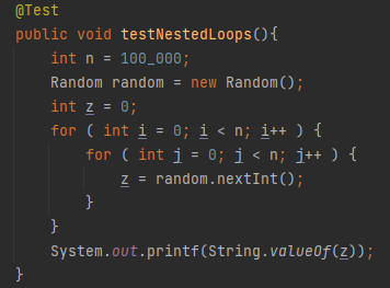
Quadratic time complexity algorithms ( O(n²)) can sometimes be optimized with better algorithms or more suitable data structures. Whenever you see a nested for loop, pay careful attention to the size of n and investigate what you can do to improve it: decrease the n, change algorithm, add bounds to input, etc., as run time can grow quite fast. If the following test runs in ~2 minutes for n = 100 000, for n = 1 000 000 it will run 1⁰² = 100 times slower which is > 3 hours, unacceptable for most applications. But as you will see later, it is not polynomial algorithms that keep us up at night. It is exponential ones.
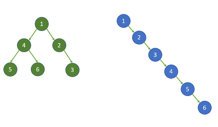
Computational complexity theory tells us what data structures to use for our business requirements if we aim to achieve the best performance. It is your duty to evaluate and understand how the users are consuming the data and what are the most common use cases. For instance, suppose your users are searching for data very often, the data size is large and searching must be done quickly, while there are less constraints on the insertion or is not that often that the data changes. In that case, you might use a Binary search tree instead of an array or a linked list, as the search and insert complexity are both O(log n), proportional to the height of the three. If the tree is unbalanced (it can have a height of n), so the complexity in the worst case can still be O(n). That is why we need to make sure that we balance the three, which involves additional operations to reconstruct sub-trees when necessary. Of course, “links” are references to objects (or memory locations), so these data structures consume more storage than an array.
No matter the data structures we choose, or the hardware we have, some algorithms are simply too difficult to to compute in a reasonable amount of time.
Classification: Deterministic vs non-deterministic
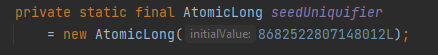
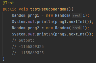
Before going further into algorithms, we are still struggling with, it is worth mentioning the distinction between deterministic and non-deterministic algorithms as well as exact or approximate ones. Deterministic algorithms always produce the same result when presented with the same input. Non-deterministic algorithms do not. Turing machines are deterministic, and consequently all our computers are the same. Well, what if you want to build an online casino? If the cards that your poker algorithm yields to the players are pre-determined, you are doomed to fail. If you happen to be a Java programmer and you cleverly thought about the infamous java.util.Random(), you are sailing in dangerous waters. To simulate non-deterministic behavior on Turing machines, Pseudo-Random Number Generators are used, simply called PRNGs. These generators use a seed number as a source, and an equation to generate numbers based on the seed. Using the same seed produces the same sequence, and eventually the sequence is repeated (hence the “pseudo”). Java Random() uses a linear congruential generator, with an equation that looks like this:
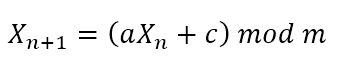
As you can see, the equation uses modulo operator, which guarantees repetition after at most m numbers, so m has to be quite big and in general a prime number is chosen, as primes don’t tend to have a ton of divisors and as such they are a good choice for a number generator based on modulo operator. The m used in our java Random() class is the mask field, a special prime number which is less then one from a power of two, which makes it easy to represent through a bitwise operation. This primes are called Mersenne primes, and are useful because they allow much faster bitwise operations for calculating the pseudo-random numbers with the above formula. Don’t you love when science meets programming?

If you keep the count, you have already noticed that primes are all over the place in computer science. The seed for java Random() class is computed using system time, as we can see by diving in the sources:
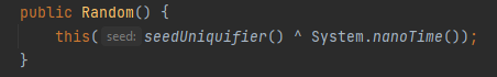
The seed “uniquifier” is just a large number that is updated at each invocation of the constructor:
Algorithms that use PRNGs are still deterministic, but they can generate numbers which statistically have similar properties with true random numbers.
If you wish to implement a fair online poker app, you need true randomness, which is hard to get. You might want to use the API of random.org: https://api.random.org/pricing, or, if you get successful and external services will get too expensive, you might want to rely on hardware that generates random numbers using thermal noise of the circuits or even better: quantum mechanics effects of small particles, which are the most random things we currently know of. However, if your app becomes extremely popular, you might find your true random generation of numbers is quite slow. Your only solution might be to combine a true random source with a pseudo-random generator that uses as a seed the true randomly generated numbers. Moreover, true RNGs usually feature asymmetries that make their outcomes not uniformly random, and you also need to apply a hash function on the randomly generated numbers. Currently used algorithms for computing a hash function collectively named SHA-2 are using block cyphers, which are also deterministic algorithms whose results appear random. The block cypher is carefully created to mix, rotate, and shift the bits in the input to produce an output “random” enough that it is impractical to reverse the operation and inside the blocks are, you guessed it: prime numbers. As you know, hash functions are now used everywhere.
There is a lot we do not know about non-deterministic algorithms, as we are still trying to understand deterministic ones. Luckily, all our computers are now deterministic (except for quantum computers). For a lot of practical applications, PRNGs algorithms can be used, with the advantages of speed, cost, ease of integration. This application includes approximation algorithms and techniques, software testing, exploration vs exploitation algorithms, etc. For some applications like cryptography, PRNGs are not consider suitable, despite continuous efforts to create cryptographically secure pseudo-random number generators.
Classification: Exact, approximate, heuristic and probabilistic algorithms
Most of the algorithms we work with in our daily work can be solved in polynomial time: searching an item in the database, sorting a list of elements, perform a payment transaction, retrieve all restaurants in your area. This class of problems is called P. A more formal definition of P is the set of all decision problems that can be solved by a Deterministic Turing Machine in polynomial time. Some of these problems are indeed hard, as the degree of polynomial can be large, or the input size can be large, and we usually can optimize them using graph theory methods (like sorted binary trees), but in general we prefer to and can find the optimal solution for them. If we compute the optimal solution, the algorithm is called “exact”.
For some problems, however, an exact algorithm is not feasible, as no algorithm is known to find the optimal solution in a reasonable amount of time. Some problems in P fall into this category, but in general this are problems for which known exact algorithms have a complexity above polynomial: exponential or factorial, both beyond our existing “Turing Machines” can compute in reasonable time even for moderate input sizes. As this is a problem we still must solve, the approach is to find polynomial algorithms that can compute approximate solutions, or “good enough” solutions to work with using heuristics based on intuition or having been observed to work in nature. As all these problems are solvable by brute force, but the run time or computing resources are impractical, we call them intractable problems. Not to be confused with unsolvable problems like the Halting problem.
An important distinction between heuristic and approximation approaches is that an approximation algorithm is provable at a bounded distance from the optimal solution, usually expressed in percentages, while for heuristics approach, we do not have a measure of how good the algorithm is, and we use it because it works. I know, it does not sound like computer “science”, but it is.
Probabilistic algorithms, also called randomized algorithms, are used both in approximation and heuristics techniques. We use probabilistic algorithms because they are simple, and because large samples of randomized data (or data generated according to a probability distribution that represents the data) can get asymptotically closer to the optimal solution given enough simple computations are executed. Usually, PRNGs are suitable for the task, so there is no need for true random generators.
Monte Carlo algorithms
Randomized algorithms have a significant role in physics related problems or in mathematics, where we are dealing with complex formulas and with inputs whose probability distribution is known. This class of algorithms is known as Monte Carlo methods, and the first practical application was the evaluation of neutron diffusion in the core of a nuclear weapon, at Los Alamos National Laboratory, in 1946. Deterministic approaches fail due to the amount of computation needed. In 1948, Monte Carlo simulations for nuclear reactions were being programmed on ENIAC, the first programmable computer ever built. Monte Carlo algorithms work because of the law of large numbers, which states that the more random trials we perform, the closer we get to the expected value of a function. As the work on nuclear fission projects was classified, this research project was named Monte Carlo, as Stanislaw Ulam’s uncle, one of the researchers involved in the project, would borrow money from relatives to gamble at Monte Carlo Casino in Monaco.
A good example of how the method works for pi approximation, as seen in the following image.
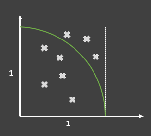
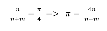
Let us illustrate the point with an algorithm you are most certainly used to.
Asymmetric cryptography
Having now a brief introduction into the history of algorithms and a few ways we can classify them, let us bridge the gap between theory and practice and put the pieces together into one of the most used algorithms today. Let us talk about asymmetric cryptography. Asymmetric cryptography, also known as public key cryptography, allows secure communication between two (or multiple) parties, while allowing the decryption of the message only by its intended receiver. This is an extreme improvement over symmetric key cryptography, where the secret (password, key) had to be shared between the two parties, which meant that both parties could decrypt the messages and each of them could pose as the other one.

The first and best-known algorithm for public key cryptography is RSA, published in ’77 by Ron Rivest, Adi Shamir, and Leonard Adleman. It is still the most used algorithm, as it has not yet been broken. You have used it many times (your browser had), whenever you sent data to a website with TLS encryption (over HTTPS). As a developer, you have generated some keys yourself. With putty, like in the image below, for SSH authentication, or self-signed SSL certificates and wondering how it works, and first, why do you have to frenetically move your mouse over the gray area.


What is happening here? If we allow ourselves to simplify a bit, we generate a public key and a private key. This two keys have to be related, so that a message encrypted with the public key can be decoded with the private key, but the private key cannot be deduced from the public key. Encryption — decryption formula in the image below relies on the difficulty of finding the number d (which is the private key) while knowing n and e (public key), as n is a product of two prime numbers, let’s call them p and q (n = pq).

Private key, d, can be computed from p and q, but to find p and q we need to decompose n into its prime factors, which is an exponential complexity algorithm (the naïve approach at least). For large enough n’s, it is highly unpractical. Current n values have 2048 bits. It seems we are back to Euclid, closing the cycle, still discussing about primes. If you have followed the discussion this far, you might have wondered: “Ok, but how do we find such huge prime numbers like p and q to begin with? Isn’t this a problem almost as hard to begin with?” And you would be right. One thing that makes prime numbers special is that we know little about their distribution. We know there’s an infinite amount of them since Euclid, but we still don’t know how to efficiently find them, except for the good old way that you’ve programed in high school: take each number (maybe skip the even ones), check if it is prime by dividing them to all primes smaller than itself (sqrt(n) would suffice as your teacher told you)). If there’s no match, you found a prime. So finding two large prime numbers is a tedious job. And obviously, we can’t use existing ones, we need new ones for each public — private key pair. This leaves us with one tradeoff option: pick to numbers at “random” and hope they are prime. Now you know enough about randomness and computers to understand why we have to move the mouse on top of the gray area. We need a “random” seed for a pseudo-random number generator used to guess to prime numbers we are searching for, p and q. That “random” is you, if you happen to believe in free will. And even if you don’t, your hand movement is still less predictable than your operating system clock. The “guess” in the equation is the Miller–Rabin primality test which is an efficient probabilistic and approximate algorithm. We can increase the probability of the number being tested to be prime by running the algorithm longer, and currently used version of it was discovered in 1980. This is yet another spooky method that seems to work well, we actually based our entire industry and security on top of it, but the proof that the Miller primality test works relies on the unproven Riemann hypothesis, probably the most famous unresolved problems in mathematics, of which I’m not smart enough to talk about. As this primality test is fast, we can quickly find two numbers that might be primes with a high enough confidence to used them in computation of the public and private keys.
Hardest problem(s) in computer science
Amongst decision problems, some problems are unsolvable (undecidable), like the halting problem. And some problems are solvable, and we know polynomial algorithms to solve them. The class of this problems is called P. There are problems for which we can verify solutions quite easy (in polynomial time). The class of this problems is called NP. For example, integer factorization, the base for our cryptography, is an NP problem. If we know the prime factors, we can quickly verify if they multiply to the result. They are named NP because all this problems can be solved in polynomial time by a Nondeterministic Turing Machine, which is a special theoretical Turing machine that can check all possible branches of an algorithm, or “guess” solutions. Obviously, P ⊂ NP. There are some decision problems however to which we can reduce any other NP problem, “root” problems if you like. This are called NP-Complete problems, and they can simulate, or solve any other problem in NP. We know quite a few of this and adding a few more to this class will bring you fame, glory and citations. And there are hard problems, which are called Hard. NP-Hard. They are at least as hard as NP-Complete, and all the problems in NP can be reduced to them in polynomial time. NP-Complete problems are a subset of NP-Hard, but some NP-Hard problems are not even in NP, or they are not decision problems.
We believe no NP-Hard problem (or NP-Complete one by inclusion) can be solved in polynomial time, as no algorithms were discovered to solve them efficiently. However, this has not yet been proven. This is the most difficult problem in computer science, and it’s called P ≠ NP. Solving this comes with eternal fame and 1 million dollars. If P were to equal NP, a lot of problems we thought are hard could be solved with a polynomial algorithm (P), meaning there are much more efficient ways to solve NP-Complete problems (and some NP-Hard ones).
The most famous NP-Complete problem is the Traveling salesman problem.

It has a factorial complexity, so solving it by brute force even for modest input size is unpractical. That is why, heuristic approaches are used instead. Most of this heuristics are randomness algorithms discussed above. For this problem, Simulated annealing does a great job, but it’s impossible to tell how good of a job it does. Another heuristic approach can be ant colony optimization, in the swarm intelligence class algorithms. Less computational ones (and also less efficient) are greedy algorithms, in which you search local optima step by step.
Brain teasers for you in the form of NP-Hard problems:
- You work at the University. New academic year starts soon and you have to assign classes to time slots so that there are no conflicts and classes for each group are as closely batched together as possible.
- You decided (or most likely finally found someone to marry to) and you need to plan your wedding. However, you know that some of your friends don’t like each other, some other’s do. Any table can have a configurable number of seats. Place your guests at the table to maximize happiness.
- Test the 6 degrees hypothesis.
- Knapsack problem: suggest articles to add to a kart (or a recommendation page) to maximize user preference match up to a certain total amount.
Machine learning algorithms
Sometimes, our problems do not involve decision, but we have to predict, model, or understand. For this type of problems, machine learning algorithms are the choice to go. It has been mathematically proven than ML algorithms as universal function approximators, so they can model anything that can be expressed as a function, provided enough neurons are defined. Deep learning is our best approach to problems where we have a lot of data, no matter how incomplete, and the output looks random. ML will find the patterns that yield the result, and possibly even more patterns (see overfitting). Pattern matching is not the hammer solution for all your nail problems, as beautifully illustrated in the following example. It has been conjectured that:

The smallest n for which the equation doesn’t hold is n=8424432925592889329288197322308900672459420460792433. Sometimes we just need better math.
I find it fascinating that our entire IT domain is based on assumption that some mathematical hypothesis might hold true, while some of the most successful algorithms we know are based on heuristics we have yet to learn how to measure. Still, with our poorly understood algorithms underneath, IT looks so smooth on the outside. So mature and scientific, yet so incomplete.

“Accesa Tech Conference”
